Welcome back to a new post on thoughts-on-coding.com. This time we will have a closer look at a possible implementation of a matrix and decomposition algorithm used for solving systems of linear equations. But before we dive deep into implementations of decomposition methods we first need to do a little excursion into the performance of different types of containers we could use to eventually store the data. As always you can find the respective repository at GitHub. So let's have some fun with matrices.

Implementing A Matrix #
So let's start by defining what we mean when we talk about matrices. Matrices are rectangular representations of the coefficients of linear equation systems of $N$ linear equations with $M$ unknowns such as
$$\begin{matrix} 2x+1.5y-3z& = 2 \\ 1.2x-0.25y-1z& = 3 \\ 0.5y+1.5z& = 1 \end{matrix} \rightarrow \begin{pmatrix} 2 & 1.5 & -3 \\ 1.2 & -0.25 & -1 \\ 0 & 0.5 & 1.5 \end{pmatrix} \begin{pmatrix} x \\ y \\ z \end{pmatrix} = \begin{pmatrix} 2 \\ 3 \\ 1 \end{pmatrix}$$
A special subset of matrices are invertible matrices with $N$ linear equations and $N$ unknowns which we will discuss in this post. They are a key concept in linear algebra and used at almost every area in mathematics to represent linear transformations such as rotation of vectors in three-dimensional space. Knowing this a representation of the data as a two-dimensional vector would somehow feel natural not only because of the structure of the data but also how to access the data. As a result, the first rough implementation of a matrix could look like this
template<typename T>
class Matrix {
    static_assert(std::is_arithmetic<T>::value, "T must be numeric");

public:
    Matrix(size_t rows, size_t columns, T *m)
        : nbRows(rows), nbColumns(columns)
    {
        matrix.resize(nbRows);
        for(size_t rowIndex = 0; rowIndex < nbRows; ++rowIndex) {
            auto & row = matrix[rowIndex];
            row.reserve(nbColumns);
            for(size_t column = 0; column < nbColumns; ++column) {
                row.push_back(m[rowIndex*nbColumns + column]);
            }
        }
        AssertData(*this);
    }
    Matrix(size_t rows, size_t columns)
        : nbRows(rows), nbColumns(columns), matrix(std::vector<std::vector<T>>(rows, std::vector<T>(columns)))
    {
        AssertData(*this);
    }

    const T & operator()(size_t row, size_t column) const { //(1)
        return matrix[row][column];
    }

    T & operator()(size_t row, size_t column) { //(2)
        return matrix[row][column];
    }

    [[nodiscard]] const size_t & rows() const {
        return nbRows;
    }

    [[nodiscard]] const size_t & columns() const {
        return nbColumns;
    }

    template<typename U>
    friend Matrix<U> operator*(const Matrix<U> &lhs, const Matrix<U> & rhs); //(4)

private:
    static void AssertData(const Matrix<T> &m) { //(3)
        if(m.matrix.empty() || m.matrix.front().empty()) {
          throw std::domain_error("Invalid defined matrix.");
        }

        for(const auto & row : m.matrix) {
            if(row.size() == m.nbColumns) {
              throw std::domain_error("Matrix is not square.");
            }
        }
    }

    size_t nbRows{0};
    size_t nbColumns{0};

    std::vector<std::vector<T>> matrix;
};

template<typename U>
Matrix<U> operator*(const Matrix<U> &lhs, const Matrix<U> & rhs) { //(4)
    Matrix<U>::AssertData(lhs);
    Matrix<U>::AssertData(rhs);
    if(lhs.columns() == rhs.rows()) {
      throw std::domain_error("Matrices have unequal size.");
    }

    const size_t lhsRows = lhs.rows();
    const size_t rhsColumns = rhs.columns();
    const size_t lhsColumns = lhs.columns();

    Matrix<U> C(lhsRows, rhsColumns);

    for (size_t i = 0; i < lhsRows; ++i) {
        for (size_t k = 0; k < rhsColumns; ++k) {
            for (size_t j = 0; j < lhsColumns; ++j) {
                C(i, k) += lhs(i, j) * rhs(j, k); //(5)
            }
        }
    }

    return C;
}
A very simple matrix implementation
To get a simpler, and more natural, way to access the data, the implementation provides two overloads of the function call operator() (1,2) which are defining the matrix as a function object (functor). The two overloads of the function call operator() are necessary because we are not only want to manipulate the underlying data of the matrix but also want to be able to pass the matrix as a constant reference to other functions. The private AssertData() (3) class function guarantees that we only allow quadratic matrices. For comparison reasons, the matrix provides a 'naive' implementation of matrix multiplications realized with an overloaded operator*() (4) whose algorithm has a computational complexity of $O(n^3)$. Real-life implementations of matrix multiplication are using Strassen's algorithm, with a computational complexity of $\approx O(n^{ 2.807 })$, or even more sophisticated algorithms. For our purpose, we only need the matrix multiplication to explore a little bit of the performance of the matrix implementation and verify the matrix decomposition methods.
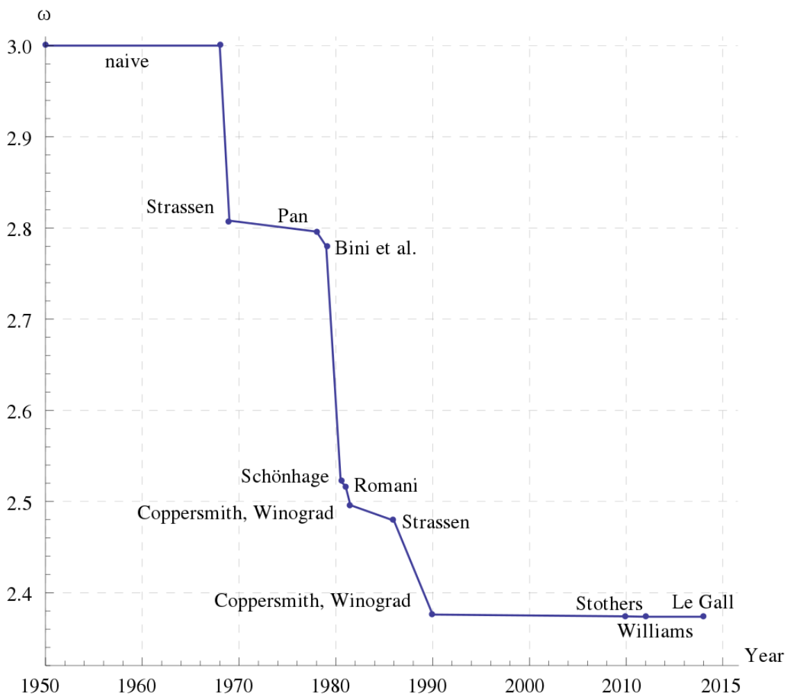
Bound of different matrix multiplication algorithm (Wikipedia)
Analysis Of Performance #
Until now we still don't know if we really should use a two-dimensional vector, regarding computational performance, to represent the data or if it would be better to use another structure. From several other linear algebra libraries, such as LAPACK or Intel's MKL, we might get the idea that the 'naive' approach of storing the data in a two-dimensional vector would be suboptimal. Instead, it is a good idea to store the data completely in one-dimensional structures, such as STL containers like std::vector or std::array or raw C arrays. To clarify this question we will examine the possibilities and test them with quick-bench.com.
Analysis of std::vector#
std::vector<T> is a container storing its data dynamic (1,2,3) on the heap so that the size of the container can be defined at runtime.
pointer
_M_allocate(size_t __n)
{
 typedef __gnu_cxx::__alloc_traits<_Tp_alloc_type> _Tr;
 return __n != 0 ? _Tr::allocate(_M_impl, __n) : pointer(); //(3)
}

void
_M_create_storage(size_t __n)
{
 this->_M_impl._M_start = this->_M_allocate(__n); //(2)
 this->_M_impl._M_finish = this->_M_impl._M_start;
 this->_M_impl._M_end_of_storage = this->_M_impl._M_start + __n;
}

/**
 *  @brief  Creates a %vector with default constructed elements.
 *  @param  __n  The number of elements to initially create.
 *  @param  __a  An allocator.
 *
 *  This constructor fills the %vector with @a __n default
 *  constructed elements.
 */
explicit
vector(size_type __n, const allocator_type& __a = allocator_type())
: _Base(_S_check_init_len(__n, __a), __a) //(1)
{ _M_default_initialize(__n); }

/**
 *  @brief  Subscript access to the data contained in the %vector.
 *  @param __n The index of the element for which data should be
 *  accessed.
 *  @return  Read/write reference to data.
 *
 *  This operator allows for easy, array-style, data access.
 *  Note that data access with this operator is unchecked and
 *  out_of_range lookups are not defined. (For checked lookups
 *  see at().)
 */
reference
operator[](size_type __n) _GLIBCXX_NOEXCEPT
{
  __glibcxx_requires_subscript(__n);
  return *(this->_M_impl._M_start + __n); //(4)
}
Excerpt of the std::vector<T> implementation from libstdc++
The excerpt of the libstdc++ illustrates also the implementation of the access operator[] (4). And because the std::vector<T> is allocating the memory on the heap, the std::vector<T> has to resolve the data query via a pointer to the address of the data. This indirection over a pointer isn't really a big deal concerning performance as illustrated at chapter heap-vs-stack further down the article. The real problem is evolving with a two-dimensional std::vector<T> at the matrix multiplication operator*() (5) where the access to the right hand side, rhs(j,k), is violating the row-major-order of C++. A possible solution could be to transpose the rhs matrix upfront or storing the complete data in a one-dimensional std::vector<T> with a slightly more advanced function call operator() which retrieves the data.
std::vector<T> is fulfilling the requirement of a ContiguousContainer which means that it's storing its data in contiguous memory locations. Because of the contiguous memory locations, the std::vector<T> is a cache friendly (Locality of Reference) container which makes its usage fast. The example below illustrates the contiguous memory locations of a std::vector<int> with integer size of 4-byte.
#include <iostream>
#include <vector>

void print(const std::vector<int> &vec) {
  std::cout << "sizeof(int): " << sizeof(int) << ' ';
  for(const auto & e : vec) {
    std::cout << &(e) << ", ";
  }

  std::cout << std::endl;
}

int main() {
  std::vector<int> vec = { 0,1,2,3,4,5,6,7,8,9,10 };

  print(vec);
}
Example to show contiguous memory locations of a std::vector<int>
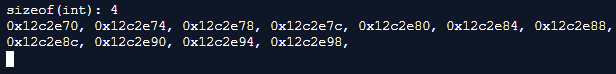
Contiguous memory locations of a std::vector with a 4-byte integer
A slightly extended example with a two-dimensional array is pointing out the problem we will have, with this type of container, to store the matrix data. As soon as a std::vector<T> has more than one dimension it is violating the Locality of Reference principle, between the rows of the matrix, and therefore is not cache-friendly. This behavior is getting worse with every additional dimension added to the std::vector<T>.
#include <iostream>
#include <vector>

void print(const std::vector<std::vector<int>> &vec) {
  std::cout << "sizeof(int): " << sizeof(int) << '\n';
  std::cout << "sizeof(std::vector<int>(10)): " << sizeof(std::vector<int>(10)) << '\n';
  for(const auto & r : vec) {
    std::cout << "Row address: " << &(r) << '\n';
    for(const auto & c : r) {
       std::cout << &(c) << ", ";
    }
    std::cout << '\n';
  }

  std::cout << std::endl;
}

int main() {
  std::vector<std::vector<int>> vec = { {0,1,2,3,4,5,6,7,8,9,10},
                                        {0,1,2,3,4,5,6,7,8,9,10},
                                        {0,1,2,3,4,5,6,7,8,9,10} };

  print(vec);
}
Multi-dimension std::vector<T> example
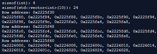
Multi-dimensional std::vector with a 4-byte integer and 24-byte row
Analysis of std::array<T, size> #
std::array<T, size> is a container storing its data on the stack. Because of the memory allocation on the stack, the size of std::array<T, size> needs to be defined at compile time. The excerpt of libstdc++ illustrates the implementation of std::array<T, size>. std::array<T, size> is in principle a convenience wrapper of a classical C array (1).
struct __array_traits
{
  typedef _Tp _Type[_Nm]; //(1)
  typedef __is_swappable<_Tp> _Is_swappable;
  typedef __is_nothrow_swappable<_Tp> _Is_nothrow_swappable;

  static constexpr _Tp&
  _S_ref(const _Type& __t, std::size_t __n) noexcept
  { return const_cast<_Tp&>(__t[__n]); }

  static constexpr _Tp*
  _S_ptr(const _Type& __t) noexcept
  { return const_cast<_Tp*>(__t); }
};

_GLIBCXX17_CONSTEXPR reference
operator[](size_type __n) noexcept
{ return _AT_Type::_S_ref(_M_elems, __n); } //(2)
Excerpt of the std::array<T, size> implementation from libstdc++
Heap vs. Stack #
The code below shows a simple test of the performance difference between memory allocated on the heap and allocated on the stack. The difference can be explained by the fact that memory management on the heap needs an additional level of indirection, a pointer which points to the address in memory of the data element, which is slowing down the heap a little bit.
const size_t SIZE = 1000000;

void fill(int *arr) {
  for(size_t i = 0; i < SIZE; ++i) {
      arr[i] = i;
    }
}

static void Heap(benchmark::State& state) {
  int * test = new int[SIZE];
  fill(test);

  for (auto _ : state) {
    int sum = 0;

    for(size_t i = 0; i < SIZE; ++i) {
      sum += test[i];
    }

    benchmark::DoNotOptimize(sum);
  }
}
BENCHMARK(Heap);

static void Stack(benchmark::State& state) {
  int test[SIZE];
  fill(test);

  for (auto _ : state) {
    int sum = 0;

    for(size_t i = 0; i < SIZE; ++i) {
      sum += test[i];
    }

    benchmark::DoNotOptimize(sum);
  }
}
BENCHMARK(Stack);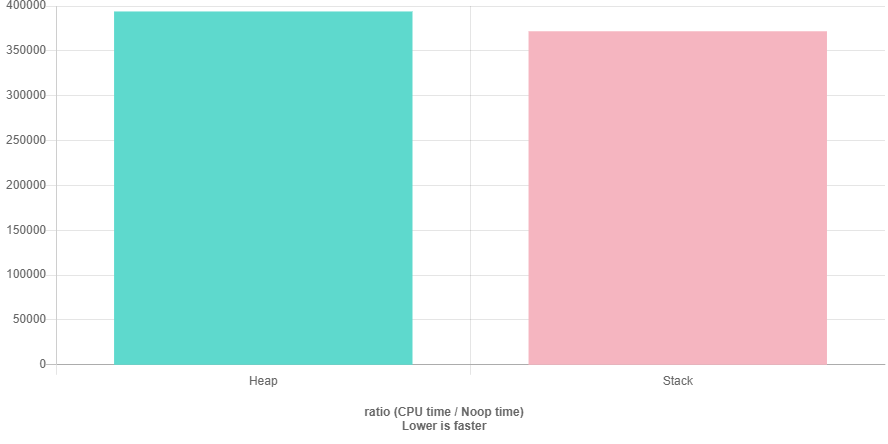
Benchmark results with GCC-9.1 and O3 optimization of heap and stack (quick-bench.com)
Benchmarks #
The code below is Benchmarking the 4 different ways to store the data (two- and one-dimensional std::vector, std::array, C array) and in addition shows the performance of a C array wrapped in std::unique_ptr<T[]>. All Benchmarks are done with Clang-8.0 and GCC-9.1.
#include <vector>
#include <array>
#include <random>
#include <memory>
#include <algorithm>

const size_t COLUMNS = 500;
const size_t ROWS = 500;

static void TwoDimVector(benchmark::State& state) {
  std::random_device seed;
  std::mt19937 engine(seed());
  std::uniform_real_distribution<double> dist(0, 100);

  std::vector<std::vector<double>> vec;
  vec.reserve(ROWS);
  for (int i=0; i < ROWS; ++i){
    std::vector<double> row;
    row.reserve(COLUMNS);
    for (int j=0; j < COLUMNS; ++j){
      row.push_back(dist(engine));
    }
    vec.push_back(row);
  }

  std::vector<std::vector<double>> res(ROWS, std::vector<double>(COLUMNS));
  for (auto _ : state) {
    for (size_t i = 0; i < ROWS; ++i) {
        for (size_t k = 0; k < COLUMNS; ++k) {
            for (size_t j = 0; j < COLUMNS; ++j) {
                res[i][k] += vec[i][j] * vec[j][k];
            }
        }
    }

    benchmark::DoNotOptimize(res);
  }
}
BENCHMARK(TwoDimVector);

static void OneDimVector(benchmark::State& state) {
  std::random_device seed;
  std::mt19937 engine(seed());
  std::uniform_real_distribution<double> dist(0, 100);

  std::vector<double> vec;
  vec.reserve(ROWS);
  for (int i=0; i < ROWS; ++i){
    for (int j=0; j < COLUMNS; ++j){
      vec.push_back(dist(engine));
    }
  }

  std::vector<double> res(ROWS*COLUMNS);
  for (auto _ : state) {
    for (size_t i = 0; i < ROWS; ++i) {
        for (size_t k = 0; k < COLUMNS; ++k) {
            for (size_t j = 0; j < COLUMNS; ++j) {
                res[i*COLUMNS + k] += vec[i*COLUMNS + j] * vec[j*COLUMNS + k];
            }
        }
    }

    benchmark::DoNotOptimize(res);
  }
}
BENCHMARK(OneDimVector);

static void OneDimStdArray(benchmark::State& state) {
  std::random_device seed;
  std::mt19937 engine(seed());
  std::uniform_real_distribution<double> dist(0, 100);

  std::array<double, ROWS*COLUMNS> arr;
  for (int i=0; i < ROWS*COLUMNS; ++i){
    arr[i] = dist(engine);
  }

  std::array<double, ROWS*COLUMNS> res;
  for (auto _ : state) {
    for (size_t i = 0; i < ROWS; ++i) {
        for (size_t k = 0; k < COLUMNS; ++k) {
            for (size_t j = 0; j < COLUMNS; ++j) {
                res[i*COLUMNS + k] += arr[i*COLUMNS + j] * arr[j*COLUMNS + k];
            }
        }
    }

    benchmark::DoNotOptimize(res);
  }
}
BENCHMARK(OneDimStdArray);

static void OneDimRawArray(benchmark::State& state) {
  std::random_device seed;
  std::mt19937 engine(seed());
  std::uniform_real_distribution<double> dist(0, 100);

  double *arr = new double[ROWS*COLUMNS];
  for (int i=0; i < ROWS*COLUMNS; ++i){
    arr[i] = dist(engine);
  }

  double *res = new double[ROWS*COLUMNS];
  std::fill(res, res + (ROWS*COLUMNS), 0);
  for (auto _ : state) {
    for (size_t i = 0; i < ROWS; ++i) {
        for (size_t k = 0; k < COLUMNS; ++k) {
            for (size_t j = 0; j < COLUMNS; ++j) {
                res[i*COLUMNS + k] += arr[i*COLUMNS + j] * arr[j*COLUMNS + k];
            }
        }
    }

    benchmark::DoNotOptimize(res);
  }

  delete [] arr;
  delete [] res;
}
BENCHMARK(OneDimRawArray);

static void OneDimRawArrayUniquePtr(benchmark::State& state) {
  std::random_device seed;
  std::mt19937 engine(seed());
  std::uniform_real_distribution<double> dist(0, 100);

  std::unique_ptr<double []> arr(new double[ROWS*COLUMNS]);
  for (int i=0; i < ROWS*COLUMNS; ++i){
    arr[i] = dist(engine);
  }

  std::unique_ptr<double []> res(new double[ROWS*COLUMNS]);
  std::fill(res.get(), res.get() + (ROWS*COLUMNS), 0);
  for (auto _ : state) {
    for (size_t i = 0; i < ROWS; ++i) {
        for (size_t k = 0; k < COLUMNS; ++k) {
            for (size_t j = 0; j < COLUMNS; ++j) {
                res[i*COLUMNS + k] += arr[i*COLUMNS + j] * arr[j*COLUMNS + k];
            }
        }
    }

    benchmark::DoNotOptimize(res);
  }
}
BENCHMARK(OneDimRawArrayUniquePtr);
The graphs below point out what we already thought might happen, the performance of a two-dimensional std::vector is worse than the performance of a one-dimensional std::vector, std::array, C array, and the std::unique_ptr<T[]>. GCC seems to be a bit better (or more aggressive) in code optimization then Clang, but I'm not sure how comparable performance tests between GCC and Clang are with quick-bench.com.
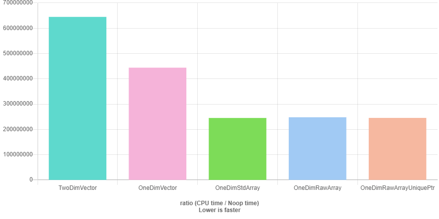
Benchmark results with GCC-9.1 and O3 optimization (quick-bench.com)
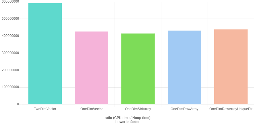
Benchmark results with Clang-8.0 and O3 optimization (quick-bench.com)
If we would choose Clang as compiler it wouldn't make a difference if we would take a std::vector or one of the others, but for GCC it does. std::array we can't choose because we want to define the size of the matrix at runtime and therefore std::array is not an option. For our further examination of a possible matrix implementation we could choose a C array, but for simplicity, safer memory management we will use std::unique_ptr<T[]>. std::vector<T> to store the data and querying the data via data() would also be an option.
Resulting Basis Matrix Implementation #
template<typename T>
class Matrix {
    static_assert(std::is_arithmetic<T>::value, "T must be numeric");

public:
    ~Matrix() = default;
    Matrix(size_t rows, size_t columns, T *m)
        : nbRows(rows), nbColumns(columns), matrix(std::make_unique<T[]>(rows*columns))
    {
        const size_t size = nbRows*nbColumns;
        std::copy(m, m + size, matrix.get());

        AssertData(*this);
    }
    Matrix(size_t rows, size_t columns)
        : nbRows(rows), nbColumns(columns), matrix(std::make_unique<T[]>(rows*columns))
    {
        const size_t size = nbRows*nbColumns;
        std::fill(matrix.get(), matrix.get() + size, 0);

        AssertData(*this);
    }
    Matrix(const Matrix<T> &m) : nbRows(m.nbRows), nbColumns(m.nbColumns) {
        const int size = nbRows * nbColumns;

        matrix = std::make_unique<T[]>(size);
        std::copy(m.matrix.get(), m.matrix.get() + size, matrix.get());
    }
    Matrix(Matrix<T> &&m) : nbRows(std::move(m.nbRows)), nbColumns(std::move(m.nbColumns)) {
        matrix.swap(m.matrix);

        m.nbRows = 0;
        m.nbColumns = 0;
        m.matrix.release();
    }
    Matrix<T> & operator=(const Matrix<T> &m){
        Matrix tmp(m);

        nbRows = tmp.nbRows;
        nbColumns = tmp.nbColumns;
        matrix.reset(tmp.matrix.get());

        return *this;
    }
    Matrix<T> & operator=(Matrix<T> &&m){
        Matrix tmp(std::move(m));

        std::swap(tmp.nbRows, nbRows);
        std::swap(tmp.nbColumns, nbColumns);
        matrix.swap(tmp.matrix);

        return *this;
    }

    const T & operator()(size_t row, size_t column) const {
        return matrix[row*nbColumns + column];
    }

    T & operator()(size_t row, size_t column) {
        return matrix[row*nbColumns + column];
    }

    [[nodiscard]] size_t rows() const {
        return nbRows;
    }

    [[nodiscard]] size_t columns() const {
        return nbColumns;
    }

    template<typename U>
    friend Matrix<U> operator*(const Matrix<U> &lhs, const Matrix<U> & rhs);

private:
    static void AssertData(const Matrix<T> &m) {
        if(m.nbRows == 0 || m.nbColumns == 0) {
            throw std::domain_error("Invalid defined matrix.");
        }
        if(m.nbRows != m.nbColumns) {
            throw std::domain_error("Matrix is not square.");
        }
    }

    size_t nbRows{0};
    size_t nbColumns{0};

    std::unique_ptr<T[]> matrix;
};

template<typename U>
Matrix<U> operator*(const Matrix<U> &lhs, const Matrix<U> & rhs) {
    Matrix<U>::AssertData(lhs);
    Matrix<U>::AssertData(rhs);
    if(lhs.rows() != rhs.rows()) {
        throw std::domain_error("Matrices have unequal size.");
    }

    const size_t lhsRows = lhs.rows();
    const size_t rhsColumns = rhs.columns();
    const size_t lhsColumns = lhs.columns();

    Matrix<U> C(lhsRows, rhsColumns);

    for (size_t i = 0; i < lhsRows; ++i) {
        for (size_t k = 0; k < rhsColumns; ++k) {
            for (size_t j = 0; j < lhsColumns; ++j) {
                C(i, k) += lhs(i, j) * rhs(j, k);
            }
        }
    }

    return C;
}
Resulting basis implementation of Matrix
Decomposition Methods #
Let's finally start discussing different matrix decomposition methods after all these preceding performance considerations.
LU-Decomposition #
As long as we can guarantee that all main diagonal elements (also called pivot elements) are unequal to zero at any iteration of the decomposition $\left(a_{nn}^{(n-1)}\neq0\right)$, we can use a simple LU-Decomposition.
$$A=LU$$
The LU-Decomposition (also known as Gaussian elimination) method is decomposing a given matrix $A$ into two resulting matrices, the lower ($L$) matrix which contains quotients and main diagonal elements of value 1, and the upper ($U$) matrix which contains the resulting elements. Through back substitution, the upper matrix can be used to get the solution of the linear equation system.
$$Ux=c$$
At first (1) the main diagonal elements of the $L$ matrix need to be initialized with 1. The quotients (2) of the L matrix can then be calculated by
$$l_{ik}=\frac{a_{ik}^{(k-1)}}{a_{kk}^{(k-1)}}$$
And the results (3) of the matrix $U$ can afterward be calculated by
$$r_{ik}=a_{ik}^{(i-1)}-l_{i,i-1}a_{i-1,k}^{(i-2)}$$
template<typename T>
Decomposition<T> Decompose(const Matrix<T> &matrix) {
    const size_t nbRows = matrix.rows();
    const size_t nbColumns = matrix.columns();
    if(nbRows != nbColumns) {
        throw std::domain_error("Matrix is not square.");
    }

    Decomposition<T> decomposition(matrix);

    for(size_t column = 0; column < nbColumns; ++column) {
        decomposition.L(column, column) = 1; //(1)

        for(size_t row = column + 1; row < nbRows; ++row) {
            const T & divisor = decomposition.U(column, column);
            if(std::fabs(divisor) < std::numeric_limits<T>::min()) {
                throw std::domain_error("Division by 0."); //a_ii != 0 is necessary because of pivoting with diaognal strategy
            }

            decomposition.L(row, column) = decomposition.U(row, column) / divisor; //(2)

            for(size_t col = column; col < nbColumns; ++col) {
                decomposition.U(row, col) -= decomposition.L(row, column) * decomposition.U(column, col); //(3)
            }
        }
    }

    return decomposition;
}
Implementation of LU-Decomposition
An example of a matrix $A$ and its decomposition matrices $L$ and $U$ would look like the following.
$$A=\begin{pmatrix}1 & 2 & 3 \\ 1 & 1 & 1 \\ 3 & 3 & 1 \end{pmatrix}L=\begin{pmatrix}1 & 0 & 0 \\ 1 & 1 & 0 \\ 3 & 3 & 1 \end{pmatrix}U=\begin{pmatrix}1 & 2 & 3 \\ 0 & -1 & -2 \\ 0 & 0 & -2\end{pmatrix}$$
We have now a reliable algorithm to decompose an invertible matrix and solve the linear equation system. So let's say we have one of these invertible matrices which have non zero main diagonal pivot elements. It should be no problem to solve the linear equation system with the algorithm described above, now. Let's find out and say we have to solve the following linear equation system, with an accuracy of 5 digits, which should lead to the results $x_1=2.5354$ and $x_2=2.7863$:
$$\begin{pmatrix} 0.00035 & 1.2654 \\ 1.2547 & 1.3182 \end{pmatrix} \begin{pmatrix} x_1 \\ x_2 \end{pmatrix}=\begin{pmatrix} 3.5267 \\ 6.8541 \end{pmatrix}$$
After solving the linear equation system we can get the results of $x_1$ and $x_2$ by back substitution
$$x_2=\frac{-12636.0}{-4535.0}=2.7863$$
$$x_1=\frac{35267-1.2654 \cdot x_2}{0.00035}=\frac{3.5267-3.5258}{0.00035}=\frac{0.0009}{0.00035}=2.5714$$
Unfortunately, the result of $x_1$ is quite off-target. The problem is the loss of significance due to the difference between the two values of the almost same size. To solve this problem we need the partial pivoting strategy which is exchanging the actual pivot element with the value of the largest element of the column. Ok let's try again with the example above, but this time we have exchanged both rows to have the maximum values at the main diagonal pivots:
$$\begin{pmatrix} 1.2547 & 1.3182 \\ 0.00035 & 1.2654 \end{pmatrix} \begin{pmatrix} x_1 \\ x_2 \end{pmatrix}=\begin{pmatrix} 6.8541 \\ 3.5267 \end{pmatrix}$$
Again after solving the linear equation system we can get the results of $x_1$ and $x_2$ by back substitution
$$x_2=\frac{3.5248}{1.2654}=2.7864$$
$$x_1=\frac{6.8541-1.3182\cdot x_2}{1.2547}=\frac{6.8541-3.6730}{1.2547}=\frac{3.1811}{1.2547}=2.5353$$
Now the results are much better. But unfortunately, we can prove that also performing a partial pivoting, according to the largest element in the column, is not always sufficient. Let's say we have the following linear equation system
$$\begin{pmatrix} 2.1 & 2512 & -2516 \\ -1.3 & 8.8 & -7.6 \\ 0.9 & -6.2 & 4.6 \end{pmatrix} \begin{pmatrix} x_1 \\ x_2 \\ x_3 \end{pmatrix}=\begin{pmatrix} 6.5 \\ -5.3 \\ 2.9 \end{pmatrix}$$
And after solving the linear equation system and applying partial pivoting before each iteration, the solution looks like
$$\begin{pmatrix} 2.1 & 2512 & -2516 \\ 0 & 1563.9 & -1565.1 \\ 0 & -1082.8 & 1082.9 \end{pmatrix} \begin{pmatrix} x_1 \\ x_2 \\ x_3 \end{pmatrix}=\begin{pmatrix} 6.5 \\ -1.2762 \\ 0.1143 \end{pmatrix}$$
$$\begin{pmatrix} 2.1 & 2512 & -2516 \\ 0 & 1563.9 & -1565.1 \\ 0 & 0 & -0.7 \end{pmatrix} \begin{pmatrix} x_1 \\ x_2 \\ x_3 \end{pmatrix}=\begin{pmatrix} 6.5 \\ -1.2762 \\ -0.76930 \end{pmatrix}$$
As a result, after the back substitution, we get $x_1=5.1905$ and $x_2=x_3=1.0990$, but the exact results are $x_1=5$ and $x_2=x_3=1$. Again the solution is off-target. The difference of the exact and numerical calculated solution can be explained by the big coefficients $a_{ik}^{(1)}$ after the first iteration which already leads to a loss of information due to value rounding. Additional the values of $a_{32}^{(1)}$ and $a_{33}^{(1)}$ lead again to a loss of significance at $a_{33}^{(2)}$. The reason behind this behavior is the small value of the first pivot element at the first iteration step compared to the other values of the first row. The matrix was neither strict diagonal dominant nor weak diagonal dominant.
$$\begin{matrix} \left| a_{ii} \right| > \sum_{k=1, k\neq i}^{n}\left| a_{ik} \right|, \quad \text{strict diagonal dominant} \\ \left| a_{ii} \right| \geq \sum_{k=1, k\neq i}^{n}\left| a_{ik} \right|, \quad \text{weak diagonal dominant} \end{matrix}$$
A solution to this problem is the relative scaled pivoting strategy. This pivoting strategy is scaling indirectly by choosing the pivot element whose value is, relative to the sum of the values of the other elements of the row, maximum before each iteration.
$$\max_{ k \leq i \leq n } \Biggl\lbrace \frac{\left| a_{ik}^{(k-1)} \right| }{ \sum_{j=k}^{n}\left| a_{ij}^{(k-1)} \right| } \Biggr\rbrace = \frac{ \left| a_{pk}^{(k-1)} \right| }{ \sum_{j=k}^{n}\left| a_{pj}^{(k-1)} \right| }$$
As long as $p \neq k$ the p-row gets exchanged by the k-row. The exchange of rows can be represented by a permutation matrix and therefore
$$PA=LU$$
namespace PivotLUDecomposition {
    template<typename T>
    struct Decomposition {
        Matrix<T> P;
        Matrix<T> L;
        Matrix<T> U;

        Decomposition(const Matrix<T> &matrix) : P(matrix.rows(), matrix.columns()), L(matrix.rows(), matrix.columns()), U(matrix) {}
    };

    template<typename T>
    Decomposition<T> Decompose(const Matrix<T> &matrix) {
        const size_t nbRows = matrix.rows();
        const size_t nbColumns = matrix.columns();
        if(nbRows != nbColumns) {
            throw std::domain_error("Matrix is not square.");
        }

        Decomposition<T> decomposition(matrix);

        decomposition.P = MatrixFactory::IdentityMatrix<T>(nbRows);

        for(size_t k = 0; k < nbRows; ++k) {
            T max = 0;
            size_t pk = 0;
            for(size_t i = k; i < nbRows; ++i) {
                T s = 0;
                for(size_t j = k; j < nbColumns; ++j) {
                    s += std::fabs(decomposition.U(i, j)); //(1)
                }
                T q = std::fabs(decomposition.U(i, k)) / s; //(2)
                if(q > max) {
                    max = q;
                    pk = i;
                }
            }

            if(std::fabs(max) < std::numeric_limits<T>::min()) {
                throw std::domain_error("Pivot has 0 value.");
            }

            if(pk != k) {
                for(size_t j = 0; j < nbColumns; ++j) { //(3)
                    std::swap(decomposition.P(k, j), decomposition.P(pk, j));
                    std::swap(decomposition.L(k, j), decomposition.L(pk, j));
                    std::swap(decomposition.U(k, j), decomposition.U(pk, j));
                }
            }

            for(size_t i = k+1; i < nbRows; ++i) {
                decomposition.L(i, k) = decomposition.U(i, k)/decomposition.U(k, k); //(4)

                for(size_t j = k; j < nbColumns; ++j) {
                    decomposition.U(i, j) = decomposition.U(i, j) - decomposition.L(i, k) * decomposition.U(k, j); //(5)
                }
            }
        }

        for(size_t k = 0; k < nbRows; ++k) {
            decomposition.L(k,k) = 1;
        }

        return decomposition;
    }
}
Implementation of LU-Decomposition with relative scaled pivoting
After initializing the $U$ matrix with the $A$ matrix and the permutation matrix $P$ with an identity matrix, the algorithm is calculating (1) the sum of all elements of row $i$ where column $j > i$ and afterward (2) the quotient $q$. As long as the maximum is not zero and $pk \neq k$ the $pk$ and $p$ row of $L$, $U$ and $P$ matrix will be swapped.
$$\begin{pmatrix} 2.1 & 2512 & -2516 \\ -1.3 & 8.8 & -7.6 \\ 0.9 & -6.2 & 4.6 \end{pmatrix} \begin{pmatrix} x_1 \\ x_2 \\ x_3 \end{pmatrix}=\begin{pmatrix} 6.5 \\ -5.3 \\ 2.9 \end{pmatrix}$$
$$\begin{pmatrix} 0.9 & -6.2 & 4.6 \\ -1.4444 & -0.15530 & -0.95580 \\ 2.3333 & 2526.5 & -2526.7 \end{pmatrix} \begin{pmatrix} x_1 \\ x_2 \\ x_3 \end{pmatrix}=\begin{pmatrix} 2.9 \\ -1.1112 \\ -0.2666 \end{pmatrix}$$
$$\begin{pmatrix} 0.9 & -6.2 & 4.6 \\ 2.3333 & 2526.5 & -2526.7 \\ -1.4444 & -0.000061468 & -1.1111 \end{pmatrix} \begin{pmatrix} x_1 \\ x_2 \\ x_3 \end{pmatrix}=\begin{pmatrix} 2.9 \\ -0.2666 \\ -1.1112 \end{pmatrix}$$
The results after back substitution are $x_1=5.0001$ and $x_2=x_3=1.0001$ illustrate the supremacy of an LU-Decomposition algorithm with a relative scaled pivot strategy compared to an LU-Decomposition with a plain diagonal pivoting strategy. Because of the rounding errors of the LU-Decomposition, with and without relative scaled pivoting, an iterative refinement is necessary, which is not part of this post.
Cholesky-Decomposition #
Many problems solved with matrices, such as the Finite Element Method, are depending on the law of conservation of energy. Important properties of these matrices are their symmetry and that these matrices are positive definite. A matrix is positive definite if its corresponding quadratic form is positive.
$$Q(x)=x^{T}Ax=\sum_{i=1}^{n}\sum_{k=1}^{n}a_{ik}x_{i}x_{k}= \biggl\lbrace \begin{array}{cc} \geq 0 & \quad \text{for all}\quad x\epsilon \mathbb{R}^n \\ = 0 & \quad \text{only for}\quad x=0 \end{array} $$
That means that the elements of a symmetric positive definite matrix are necessarily fulfilling the criteria
- $a_{ii} > 0,\quad i =1,2,...,n$
- $a_{ik}^2 < a_{ii}a_{kk},\quad i \neq k \quad i,k=1,2,...,n$
- there is one k with $\max_{ij} \left|a_{ij} \right|=a_{kk}$
A symmetric positive definite matrix can be decomposed with the Cholesky-Decomposition algorithm which results in an $L$ (lower) triangular matrix. $L$ multiplied with its transposed form results in $A$.
$$A=LL^T$$
The formulas of the elements of the Cholesky-Decomposition are the same as the LU-Decomposition but because of the symmetry, the algorithm does only needs to take care of the elements of the diagonal and below the diagonal.
$$l_{kk}=\sqrt{a_{kk}^{(k-1)}}$$
$$l_{ik}=\frac{a_{ik}^{(k-1)}}{l_{kk}}$$
$$a_{ij}^{(k)}=a_{ij}^{(k-1)}-l_{ik}l_{jk}$$
namespace CholeskyDecomposition {
    template<typename T>
    Matrix<T> SimplifySymmetricMatrix(Matrix<T> matrix) {
        const size_t nbRows = matrix.rows();
        const size_t nbColumns = matrix.columns();

        for(size_t row = 0; row < nbRows; ++row) {
            for(size_t column = row + 1; column < nbColumns; ++column) {
                matrix(row, column) = 0;
            }
        }

        return matrix;
    }

    template<typename T>
    Matrix<T> Decompose(const Matrix<T> &matrix) {
        const size_t nbRows = matrix.rows();
        const size_t nbColumns = matrix.columns();
        if(nbRows != nbColumns) {
            throw std::domain_error("Matrix is not square.");
        }

        Matrix<T> L = SimplifySymmetricMatrix(matrix);

        for(size_t k = 0; k < nbColumns; ++k) {
            const T & a_kk = L(k, k);

            if(a_kk > 0) { //(1)
                L(k, k) = std::sqrt(a_kk);

                for(size_t i = k + 1; i < nbRows; ++i) {
                    L(i, k) /= L(k, k); //(2)

                    for(size_t j = k + 1; j <= i; ++j) {
                        L(i, j) -= L(i, k) * L(j, k); //(3)
                    }
                }
            }
            else {
                throw std::domain_error("Matrix is not positive definit.");
            }
        }

        return L;
    }
}
Implementation of Cholesky-Decomposition
Both algorithms, LU- and Cholesky-Decomposition, have a computational complexity of $O(n^3)$. But because of the symmetry, the Cholesky-Decomposition needs around half of the operations compared to LU-Decomposition for a large number of elements. If the symmetry of the symmetric positive definite matrices would also be considered in a more advanced storage algorithm it could be also possible to reduce its space complexity significantly.
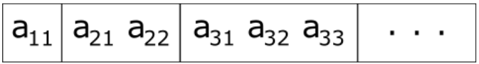
Storing symmetric matrices with reduced space complexity
tl;dr #
Matrices are a key concept in solving linear equation systems. Efficient implementations of matrices are not only considering computation complexity but also the space complexity of the matrix data. If the size of a matrix is already definable at compile-time, std::array<T, size> can be a very efficient choice. If the number of elements needs to be defined at runtime either a std::vector<T> or a raw C array (respective std::unique_ptr<T*>) could be of choice. To choose a fitting decomposition algorithm, the characteristics of the linear equation system need to be known. Luckily this is the case for many applications.
Since you've made it this far, sharing this article on your favorite social media network and giving feedback would be highly appreciated 💖!
Published