Welcome back to a new post at thoughts-on-coding.com. In this post, I would like to discuss the Gauss integration algorithm, more precisely the Gauss-Legendre integration algorithm. The Gauss-Legendre integration is the most known form of the Gauss integrations.
Others are
- Gauss-Tschebyschow
- Gauss-Hermite
- Gauss-Laguerre
- Gauss-Lobatto
- Gauss-Kronrod
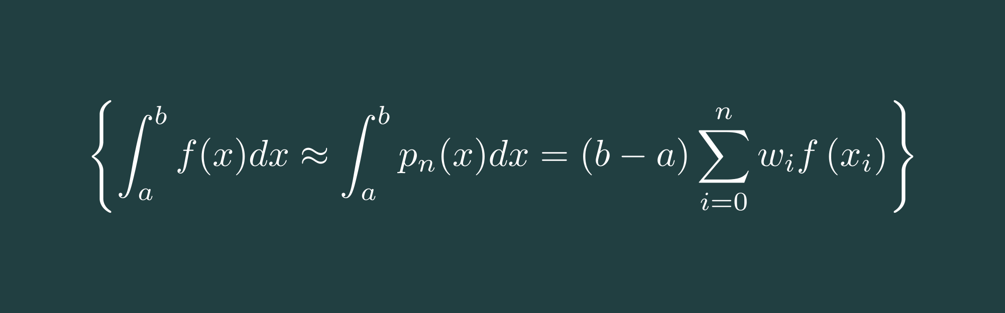
The idea of the Gauss integration algorithm is to approximate, similar to the Simpson Rule, the function $f(x)$ by
$$f(x)=w(x) \cdot \phi (x)$$
While $w(x)$ is a weighting function, $\phi(x)$ is a polynomial function (Legendre-Polynomials) with defined nodes $x_i$ which can be exactly integrated. A general form for a range of a-b looks like the following.
$$\int_{a}^{b} f(x) \mathrm{d} x \approx \frac{b-a}{2} \sum_{i=1}^{n} f\left(\frac{b-a}{2} x_{i}+\frac{a+b}{2}\right) w_{i}$$
The Legendre-Polynomials are defined by the general formula and its derivative
$$P_n(x)=\sum_{k=0}^{n/2}=(-1)^k\frac{(2n-2k)!}{(n-k)!(n-2k)!k!2^n}x^{n-2k}$$
$$P_{n}^{\prime}(x)=\frac{n}{x^{2}-1}\left(x P_{n}(x)-P_{n-1}(x)\right)$$
The following image is showing the 3rd until the 7th Legendre Polynomials, the 1st and 2nd polynomials are just 1 and x and therefore not necessary to show.
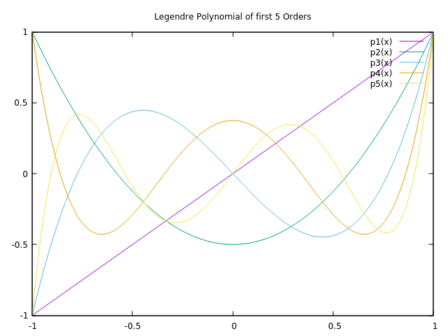
This diagram shows the first 5 orders of the Legendre Polynomial except order 0.
Let's have a closer look at the source code:
class LegendrePolynomial {
public:
    LegendrePolynomial(double lowerBound, double upperBound, size_t numberOfIterations)
        : mLowerBound(lowerBound), mUpperBound(upperBound), mNumberOfIterations(numberOfIterations), mWeight(numberOfIterations+1), mRoot(numberOfIterations+1) {
        calculateWeightAndRoot();
    }

    const std::vector<double> & getWeight() const {
        return mWeight;
    }

    const std::vector<double> & getRoot() const {
        return mRoot;
    }

private:
    const static double EPSILON;

    struct Result {
        double value;
        double derivative;

        Result() : value(0), derivative(0) {}
        Result(double val, double deriv) : value(val), derivative(deriv) {}
    };

    void calculateWeightAndRoot() {
        for(int step = 0; step <= mNumberOfIterations; step++) {
            double root = cos(M_PI * (step-0.25)/(mNumberOfIterations+0.5));
            Result result = calculatePolynomialValueAndDerivative(root);

            double newtonRaphsonRatio;
            do {
                newtonRaphsonRatio = result.value/result.derivative;
                root -= newtonRaphsonRatio;
                result = calculatePolynomialValueAndDerivative(root);
            } while (fabs(newtonRaphsonRatio) > EPSILON);

            mRoot[step] = root;
            mWeight[step] = 2.0/((1-root*root)*result.derivative*result.derivative);
        }
    }

    Result calculatePolynomialValueAndDerivative(double x) {
        Result result(x, 0);

        double value_minus_1 = 1;
        const double f = 1/(x*x-1);
        for(int step = 2; step <= mNumberOfIterations; step++) {
            const double value = ((2*step-1)*x*result.value-(step-1)*value_minus_1)/step;
            result.derivative = step*f*(x*value - result.value);

            value_minus_1 = result.value;
            result.value = value;
        }

        return result;
    }

    const double mLowerBound;
    const double mUpperBound;
    const int mNumberOfIterations;
    std::vector<double> mWeight;
    std::vector<double> mRoot;
};

const double LegendrePolynomial::EPSILON = 1e-15;

double gaussLegendreIntegral(double a, double b, int n, const std::function<double (double)> &f) {
    const LegendrePolynomial legendrePolynomial(a, b, n);
    const std::vector<double> & weight = legendrePolynomial.getWeight();
    const std::vector<double> & root = legendrePolynomial.getRoot();

    const double width = 0.5*(b-a);
    const double mean = 0.5*(a+b);

    double gaussLegendre = 0;
    for(int step = 1; step <= n; step++) {
        gaussLegendre += weight[step]*f(width * root[step] + mean);
    }

    return gaussLegendre * width;
}
The integral is done by the gaussLegendreIntegral (line 69) function which is initializing the LegendrePolynomial class and afterward solving the integral (line 77 - 80). Something very interesting to note: We need to calculate the Legendre-Polynomials only once and can use them for any function of order n in the range a-b. The Gauss-Legendre integration is therefore extremely fast for all subsequent integrations.
The method calculatePolynomialValueAndDerivative is calculating the value (line 50) at a certain node $x_i$ and its derivative (line 51). Both results are used at method calculateWeightAndRoot to calculate the the node $x_i$ by the Newton-Raphson method (line 33 - 37).
$$x_{n+1}=x_{n}-\frac{f\left(x_{n}\right)}{f^{\prime}\left(x_{n}\right)}$$
The weight $w(x)$ will be calculated (line 40) by
$$w_{i}=\frac{2}{\left(1-x_{i}^{2}\right)\left[P_{n}^{\prime}\left(x_{i}\right)\right]^{2}}$$
As we can see in the screen capture below, the resulting approximation of
$$I=\int_0^{\pi/2} \frac{5}{e^\pi-2}\exp(2x)\cos(x)dx=1.0$$
is very accurate. We end up with an error of only $-3.8151e^{-6}$. Gauss-Legendre integration works very good for integrating smooth functions and result in higher accuracy with the same number of nodes compared to Newton-Cotes Integration. A drawback of Gauss-Legendre integration might be the performance in case of dynamic integration where the number of nodes are changing.
*Screen capture of program execution*Since you've made it this far, sharing this article on your favorite social media network and giving feedback would be highly appreciated 💖!
Published