Welcome to a new post on thoughts-on-coding.com. This time I would like to start a new series, Numerical Methods. But don't be disappointed if you're expecting a new post on the n-body-problem, I'm still planning to continue the "My God, It's Full of Stars" series. With this new series, I would like to talk about numerical methods which are important in my daily business, starting from Trapezoidal and Simpson integration methods of type Newton-Cotes.
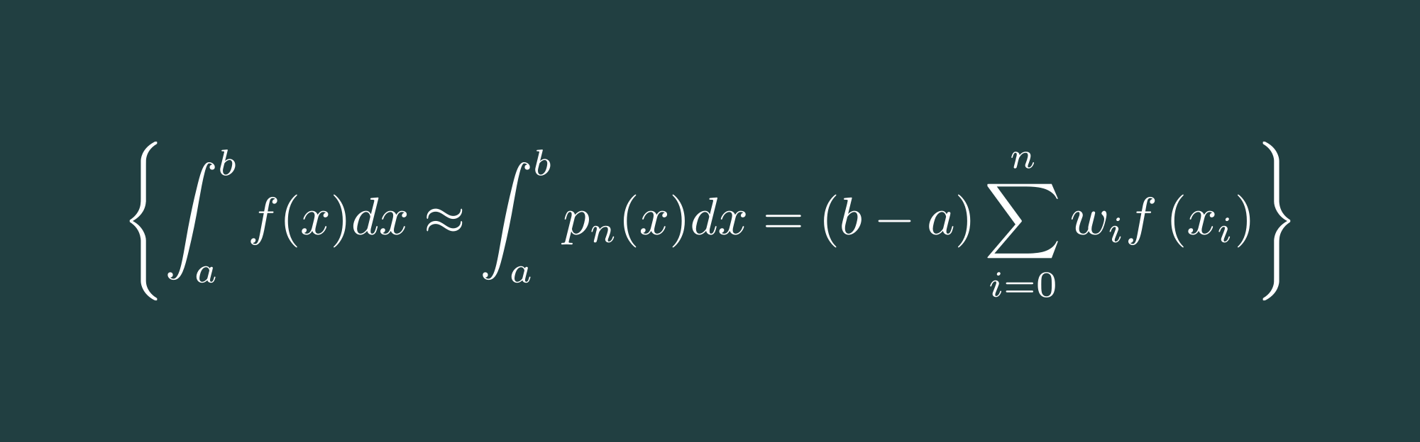
The Newton-Cotes formula is a quadratic numerical approximation for integral calculations. The idea is to interpolate the function, which shall be integrated, by a polynomial with equidistant nodes. The polynomial can be of, for example, a form of aligned trapezoids or aligned parables. Common Newton-Cotes integration polynomial rules are
- Trapezoid rule
- Simpson rule
- Romberg
- Pulcherrima
- Milne/Boole rule
- 6-Node rule
- Weddle rule
With this post, we will have a closer look at the first two integration rules, Trapezoidal and Simpson.
Trapezoidal Integral Approximation #
The integral approximation by trapezoids is very simple to explain. All we need to do is to subdivide the example function
$$I=\int_0^{\pi/2} \frac{5}{e^\pi-2}\exp(2x)\cos(x)dx=1.0$$
we want to integrate into equidistant areas whose exact integrations we can sum up. Clearly, the accuracy of the approximation is depending on the number of subdivisions N. The width of each area is therefore defined by
$$\Delta x = \frac{b-a}{N}$$
with $a=0$ and $b=\pi/2$.
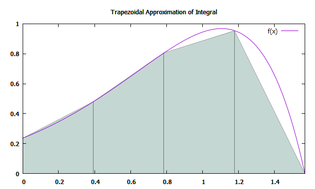
Approximation of integral of $f(x)$ between 0 and $\frac{\pi}{2}pi$ by trapezoids
The area of each trapezoid can be calculated by
$$A=\frac{a+b}{2}\cdot h$$
and therefore the approximated integral $\widetilde{ I }$ of our function $f(x)$ can be defined as
$$\widetilde{ I } = \sum_{i=1}^{N+1} \frac{x_i-x_{i+1}}{2}(f(x_i)+f(x_{i+1}))$$
The implementation of the Trapezoidal integration is taking 4 parameters, the range $[a,b]$ of integration of the function $f(x)$, the number of subdivisions $n$, and the function $f(x)$.
double trapezoidalIntegral(double a, double b, int n, const std::function<double (double)> &f) {
    const double width = (b-a)/n;

    double trapezoidal_integral = 0;
    for(int step = 0; step < n; step++) {
        const double x1 = a + step*width;
        const double x2 = a + (step+1)*width;

        trapezoidal_integral += 0.5*(x2-x1)*(f(x1) + f(x2));
    }

    return trapezoidal_integral;
}
Simpson Integral Approximation #
The Simpson rule is approximating the integral of the function $f(x)$ by the exact integration of a parable $p(x)$ with nodes at $a$, $b$, and $m=\frac{a+b}{2}$. In order to increase the approximation accuracy, the function can be subdivided by $N$, similar to the Trapezoidal integral approximation.
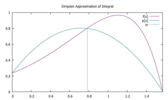
Approximation of integral of $f(x)$ between 0 and $\frac{\pi}{2}pi$ by a parabola
The exact integration can be done by summing up the area of 6 rectangles with equidistant width. The height of the first rectangle is defined by $f(x_a)$, the height of the next 4 rectangles is defined by $f(\frac{a+b}{2})$, and the height of the last rectangle is defined by $f(x_b)$. As a result, the formula of the approximated integral according to Simpson rule can be defined as
$$\widetilde{ I } = \sum_{i=1}^{N+1} \frac{x_i-x_{i+1}}{6}(f(x_i)+4f(\frac{a+b}{2})+f(x_{i+1}))$$
The implementation of the Simpson integration is, similar to the Trapezoidal based solution, taking 4 parameters, the range $[a,b]$ of integration of the function $f(x)$, the number of subdivisions $n$, and the function $f(x)$
double simpsonIntegral(double a, double b, int n, const std::function<double (double)> &f) {
    const double width = (b-a)/n;

    double simpson_integral = 0;
    for(int step = 0; step < n; step++) {
        const double x1 = a + step*width;
        const double x2 = a + (step+1)*width;

        simpson_integral += (x2-x1)/6.0*(f(x1) + 4.0*f(0.5*(x1+x2)) + f(x2));
    }

    return simpson_integral;
}
Romberg Integral Approximation #
If we integrate the function $f(x)$ with the Trapezoidal approach but bisecting the step size based on the step size of the previous step, we get the approximation sequence
$$T(1)=0.18755, > T(\frac{1}{2})=0.724727, > T(\frac{1}{4})=0.925565$$
The idea of the Romberg integration is now to introduce a y-axis symmetric parable which is crossing the points $T(1), > T(\frac{1}{2})$ and extrapolate to $x \rightarrow 0$.
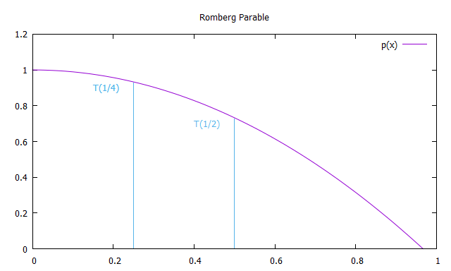
Romberg parable with nodes at T(1/2) and T(1/4)
Therefore every term of the first column $R(n,0)$ of the Romberg integration is equivalent to the Trapezoidal integration, were every solution of the second column $R(n,1)$ is equivalent to the Simpson rule, and every solution of the third column $R(n,2)$ is equivalent to Boole's rule. As a result, the Formulas for the Romberg integration are
$$R(0,0)=h_{1}(f(a)+f(b))$$
$$R(n, 0)=\frac{1}{2} R(n-1,0)+h_{n} \sum_{k=1}^{2^{\pi-1}} f\left(a+(2 k-1) h_{n}\right)$$
$$R(n, m)=R(n, m-1)+\frac{R(n, m-1)-R(n-1, m-1)}{4^{m}-1}$$
std::vector<std::vector<double>> rombergIntegral(double a, double b, size_t n, const std::function<double (double)> &f) {
    std::vector<std::vector<double>> romberg_integral(n, std::vector<double>(n));

    //R(0,0) Start with trapezoidal integration with N = 1
    romberg_integral.front().front() = trapezoidalIntegral(a, b, 1, f);

    double h = b-a;
    for(size_t step = 1; step < n; step++) {
        h *= 0.5;

        //R(step, 0) Improve trapezoidal integration with decreasing h
        double trapezoidal_integration = 0;
        size_t stepEnd = pow(2, step - 1);
        for(size_t tzStep = 1; tzStep <= stepEnd; tzStep++) {
            const double deltaX = (2*tzStep - 1)*h;
            trapezoidal_integration += f(a + deltaX);
        }
        romberg_integral[step].front() = 0.5*romberg_integral[step - 1].front() + trapezoidal_integration*h;

        //R(m,n) Romberg integration with R(m,1) -> Simpson rule, R(m,2) -> Boole's rule
        for(size_t rbStep = 1; rbStep <= step; rbStep++) {
            const double k = pow(4, rbStep);
            romberg_integral[step][rbStep] = (k*romberg_integral[step][rbStep-1] - romberg_integral[step-1][rbStep-1])/(k-1);
        }
    }

    return romberg_integral;
}The repository numericalIntegration can be found at GitHub. It will also contain the other numerical integration methods, as the name suggests, later on.
Since you've made it this far, sharing this article on your favorite social media network and giving feedback would be highly appreciated 💖!
Published